Table Of Content
These graph templates are designed to be compatible with WPS Spreadsheet, a Microsoft Excel alternative. One of the key advantages of Excel dashboards is their ability to present data in a visually engaging manner. By incorporating visual elements such as icons, shapes, and charts, you can transform your dashboard from a static grid of numbers into an interactive, informative tool. When designing your layout, consider the specific needs and preferences of your target audience.
Chart Mistake 1: Redundant Information using PowerPoint or Excel Charts
To do so, you can select the Maximum option — two fields down under Bounds in the Format Axis window — and change the value from 0.6 to one. Here, you can decide if you want to display units located on the Axis Options tab. You can change whether the Y-axis shows percentages to two decimal places or no decimal places. Once you‘ve created your chart, you’ll want to size those labels up so they're legible. Sometimes, you’ll see that your information just presents better one way versus the other.
Follow Excel Easy
This template helps to build easy-to-understand and professional-looking organizational charts that can fully represent your company’s structure. The Vertex42 website is a vast resource for Excel templates of all sorts, including a specific Pareto Chart Template. Pareto Charts are extremely helpful in identifying major problems or causes in data analysis as they sort categories by the count of their occurrences. The Vertex42 Pareto Chart Template helps you simplify the steps in creating these insightful visualizations. You can find them in the template gallery within Excel, which provides a basic framework for creating and customising your Gantt chart to fit specific project needs. 4) Ensure Data Labels for this data series are shown by clicking the Chart Elements icon at the top right of the chart.
Recommended Reads
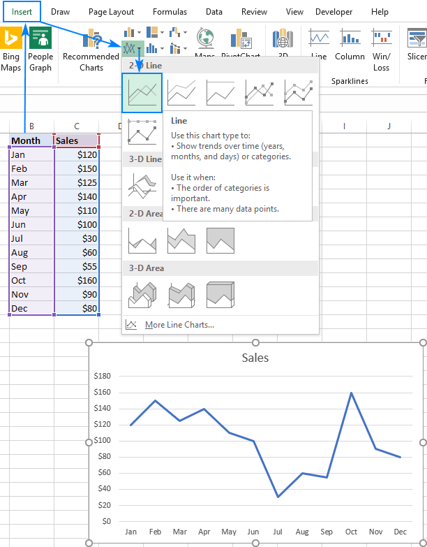
And for the rest of the tutorial, we will focus on the most recent versions of Excel. After selecting the graph type, Excel will automatically generate the graph based on your data. Next, click on the ‘Insert’ tab and select the type of graph you want to create from the Charts group.
How to Create a Histogram in Excel for Windows or Mac - Lifewire
How to Create a Histogram in Excel for Windows or Mac.
Posted: Sun, 24 Apr 2022 07:00:00 GMT [source]
Chart Mistake 3: Lack of Focus
Select your chart again and repeat the process to see your data on as many types of charts as you’d like. Because my graph automatically sets the Y axis' maximum percentage to 60%, you might want to change it manually to 100% to represent data on a universal scale. To further format the legend, click on it to reveal the Format Legend Entry sidebar, as shown below.
Business Charts in Excel
A new chart can also be inserted without having to highlight your data beforehand. To insert a chart, highlight the entire table including the headers. Given a set of data shown below, there are several ways to insert a new chart.
Chart Mistake 5: Poor Color Choices in PowerPoint Graphs
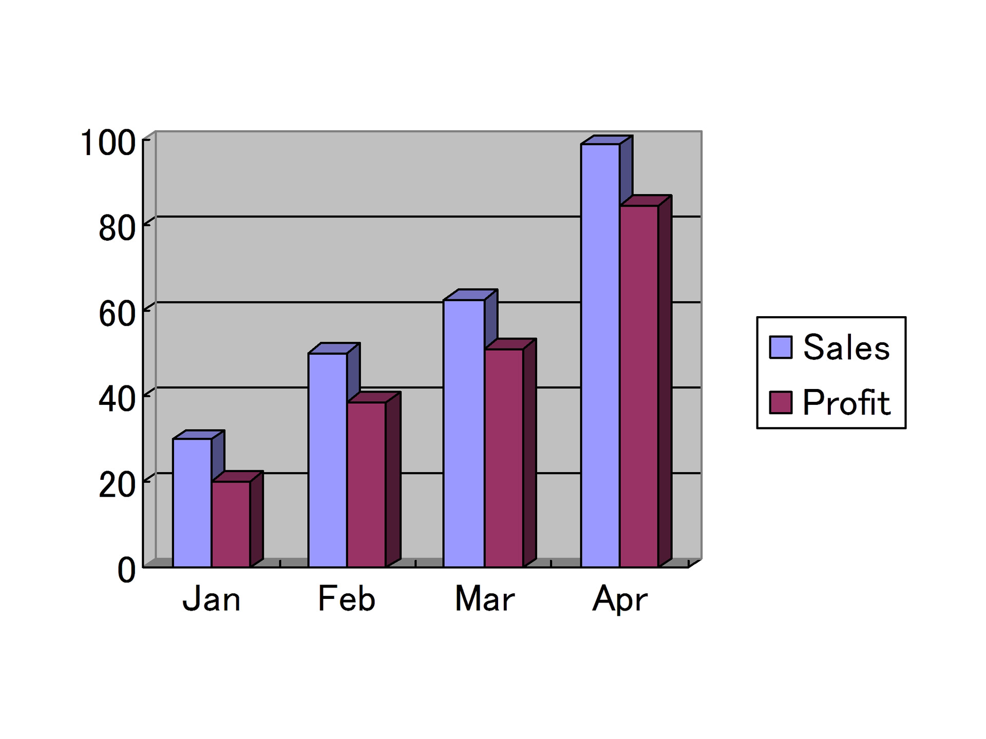
A scatter plot, also called a coordinate graph, uses dots to represent the data values for two different variables, one on each axis. This graph is used to find a pattern/ relationship between two sets of data. A line graph is formed by connecting a series of values/data points using straight lines. A line graph can be used when you want to check whether the values are increasing or decreasing over some time. To move the legend to the right side of the chart, execute the following steps. In this example, I placed the Sales series data labels on the Inside Base, while the Budget series data labels are placed Above.
Tips: Excel Graph Creation
Whether you’re a student, business professional, or just someone who loves organizing data, mastering the art of graph-making in Excel will elevate your data presentation game. In this article, we’ll walk you through the simple steps to create eye-catching graphs that will make your data pop and keep your audience engaged. Pie graphs usually compare parts of a whole, while bar graphs can compare pretty much anything ...
How to Create a Timeline in Excel - Lifewire
How to Create a Timeline in Excel.
Posted: Wed, 02 Dec 2020 08:00:00 GMT [source]
Moving, formatting or hiding the chart legend
To master Excel, enhancing your formula writing skills is essential. Implementing key tips and tricks can significantly minimize errors, such as understanding operation precedence and utilizing Excel’s built-in error-checking tools. These practices not only improve the accuracy of your calculations but also streamline your workflow, helping you manage data more effectively and with confidence.
Next, double-click the shaded area on the chart (in this case, the red area) and a "Format Data Series" menu will appear. Click on "Fill" from the lefthand side, and choose "Solid Fill." Under "Fill Color," choose the same color as the line in the chart. You can change the transparency to whatever you'd like -- a transparency of 66% looks good. A line of a different color (in this case, red) will appear on top of our original line on the chart.
Of course, this article has only scratched the surface of Excel chart customization and formatting, and there is much more to it. In the next tutorial, we are going to make a chart based on data from several worksheets. And in the meanwhile, I encourage you to review the links at the end of this article to learn more. To edit a data series, click the Edit Series button to the right of the data series. The Edit Series button appears as soon as you hover the mouse on a certain data series. This will also highlight the corresponding series on the chart, so that you could clearly see exactly what element you will be editing.
Whether you're using Windows or macOS, creating a graph from your Excel data is quick and easy, and you can even customize the graph to look exactly how you want. This wikiHow tutorial will walk you through making a graph in Excel. Because graphs and charts serve similar functions, Excel groups all graphs under the “chart” category. In this article, we’ll give you a step-by-step guide to creating a chart or graph in Excel 2016. It is crucial to choose the appropriate graph type that best represents the data being presented. Selecting the wrong type of graph can lead to misinterpretation of the data and convey inaccurate information.
This is especially true if you have imported the data from a third-party application. Generally, this type of information is not filtered of redundancies. And you might end up corrupting the integrity of your information if duplicates sneak into your pictorial representation of trends. When working with copious volumes of data, it is best to use the Remove Duplicates option on your rows. If you are looking to take note of trends over time then Line graphs are your best bet. The first step is to actually populate an Excel spreadsheet with the data that you need.
The first thing to know is that you can create different types of charts and graphs in the software. I see that this color choice is often caused by a badly designed PPT palette. When you add a data chart in MS PowerPoint or MS Excel, it uses a color palette that you have predefined in your template. If those colors are too similar, your default data chart will look less readable. You can update chart colors manually, however, I recommend updating the whole color palette, if it’s possible for you.
A simple chart in Excel can say more than a sheet full of numbers. Find the series that seems to be invisible, select it and adjust formatting. If you have multiple series, you have the option of rearranging them on the chart. This will display the Edit Series window where you will need to specify the Series name and the Series values, in our case – the Budget column header and Budget values. Alternatively, right-mouse click on the axis labels and select Font. Right-click on the chart element and specify the colors you prefer from the fly-out menu.
A chart, also known as graph, is a graphical representation of numeric data where the data is represented by symbols such as bars, columns, lines, slices, and so on. It is common to make graphs in Excel to better understand large amounts of data or relationship between different data subsets. Proper labeling and titling of the graph are essential for clarity and comprehension. Failing to label the axes, provide a clear title, and add a legend can confuse the audience and diminish the impact of the graph. Be sure to include all necessary labels and titles to ensure the graph is easily understood.


No comments:
Post a Comment